Signal versus noise
Distinguish meaningful information from random fluctuation. Set thresholds and smoothing to avoid reacting to noise, and act only when movements clear expected variability.
author
General usage across stats, engineering, finance
Model type

About
Every metric mixes signal (systematic effect) with noise (random variation, measurement error, short-term churn). Decisions improve when you size typical variation first, then require movements to exceed it before you change course.
How it works – what to map
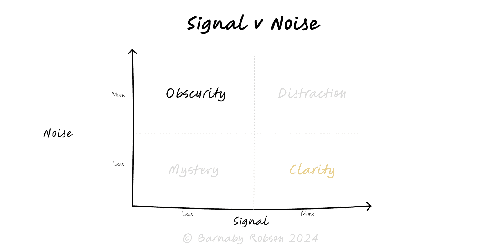
Signal – consistent pattern caused by a mechanism (trend, seasonality, causal impact).
Noise – random/unsystematic variation from sampling, timing, or measurement error.
Signal-to-noise ratio (SNR) – strength of effect vs variance; low SNR needs more data or stronger designs.
Smoothing/aggregation – moving averages, EWMA, weekly cohorts reduce noise to reveal trend.
Control limits – define expected bounds (e.g. ±3σ). Points outside likely indicate signal.
Bias–variance trade-off – more smoothing reduces variance but can hide real changes (lag).
Multiple comparisons – many metrics/tests inflate false positives; control with pre-specification or correction.
Use cases
Dashboards – show trend + control limits so leaders don’t chase random wiggles.
A/B tests – require pre-set power, minimum detectable effect, and stopping rules.
Forecasting – decompose time series (trend/seasonality/residual) before modelling.
Ops quality – SPC charts to detect real process shifts vs common-cause variation.
Investment & diligence – distinguish narrative noise from persistent unit-economic shifts.
How to apply
Define the question and horizon (daily noise tolerable, weekly actionable?).
Baseline variability – estimate typical range (σ/IQR) or seasonality pattern.
Set detection rules – e.g. “act if 2 consecutive weeks outside control limits”.
Smooth appropriately – use 7-day/28-day averages or cohort windows aligned to behaviour.
Pre-commit – metrics, MDE, duration; avoid peeking and KPI-shopping.
Instrument decisions – log when a move was triggered by signal and measure post-effect.
pitfalls and cautions
Chasing wiggles – reacting within expected variance (common-cause).
Bad denominators – ratio changes from traffic mix masquerade as signal.
Seasonality confusion – weekly/holiday effects misread as trends.
Multiple testing – fishing across many cuts inflates false positives.
Over-smoothing – hiding real step-changes; review lag vs sensitivity.
Bad denominators – ratio changes from traffic mix masquerade as signal.
Seasonality confusion – weekly/holiday effects misread as trends.
Multiple testing – fishing across many cuts inflates false positives.
Over-smoothing – hiding real step-changes; review lag vs sensitivity.