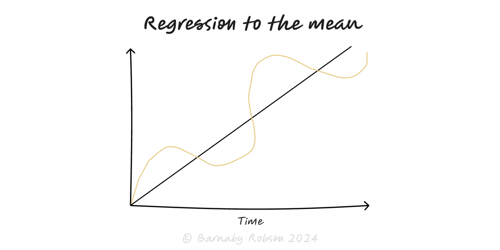
Regression to the Mean
Extreme results are usually followed by more typical ones—even without any real change.
Author
Francis Galton (1886); modern statistics and epidemiology
Model type
Extreme results are usually followed by more typical ones—even without any real change.
Francis Galton (1886); modern statistics and epidemiology
Regression to the mean is a statistical tendency: when outcomes vary and today’s result is unusually high or low, the next measurement is likely to be closer to average simply because luck/noise won’t be extreme twice in a row. Galton noticed tall parents had tall—but less extreme—children on average. It’s not a force pushing outcomes; it’s a sampling effect that fools us into seeing causation (e.g., “the cure worked!”) where none exists.
Conditions – there’s genuine variability and the correlation between time-1 and time-2 is imperfect (r < 1).
Expectation – E[X_{2}\,|\,X_{1}=x] \approx \mu + r\,(x-\mu); with 0<r<1, the expected follow-up is nearer the mean \mu.
Selection on extremes – if you pick the worst performers or the best funds, their later scores will look better/worse even without intervention.
Illusory improvement – any programme targeted at extreme cases will appear to “work” unless you control for this effect.
Performance & sport – “hot hands”, “SI jinx”, star funds; extreme runs cool naturally.
Product & ops – teams targeted after a bad month will often rebound anyway.
Medicine & policy – treat only the highest BP/lowest scores and you’ll overstate treatment effects.
A/B testing & analytics – picking variants after a lucky spike leads to disappointment on reruns.
Quality control – outlier weeks drift back without any process change.
Use proper controls – randomise or add a matched control group so both groups regress similarly.
Measure multiple baselines – average several pre-tests to reduce noise before intervening.
Analyse deltas, not levels – difference-in-differences or ANCOVA (post adjusted for pre) rather than raw post.
Shrink extreme estimates – use Bayesian/hierarchical models or empirical Bayes to temper outliers.
Beware “coach effect” stories – if you intervene because results were extreme, expect improvement even if the intervention is useless.
Report uncertainty – show intervals, reliability (r), and rerun on new samples.
Forecast sanely – temper peaks/troughs toward typical levels unless you have a causal reason not to.
Mistaking reversion for remedy – crediting training, penalties or bonuses for natural bounce-backs.
One-group pre/post – classic trap; without controls you mostly measure regression.
Overfitting – picking the best model/creator/fund from many ensures a later slide.
Changing variance – if measurement noise or mix shifts, the amount of regression changes.
Punishing extremes – regression makes “punishment works, praise fails” look true (Kahneman note); design fair feedback loops.
Click below to learn other mental models

Before building, map the space: the key forks, dead ends and dependencies—so you can choose a promising path and run smarter tests.
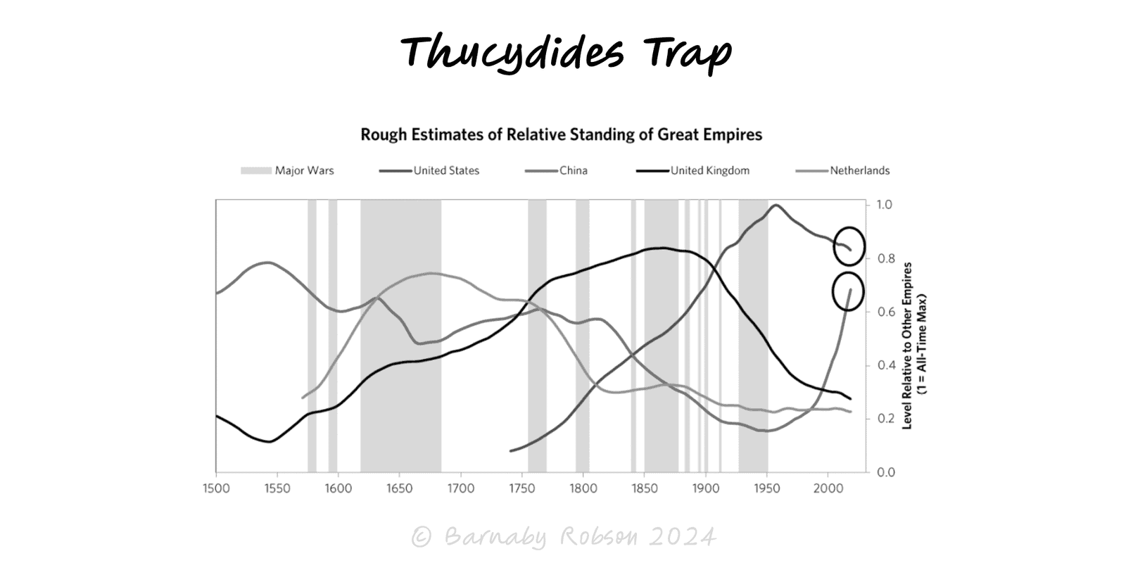
When a rising power threatens to displace a ruling power, fear and miscalculation can tip competition into conflict unless incentives and guardrails are redesigned.
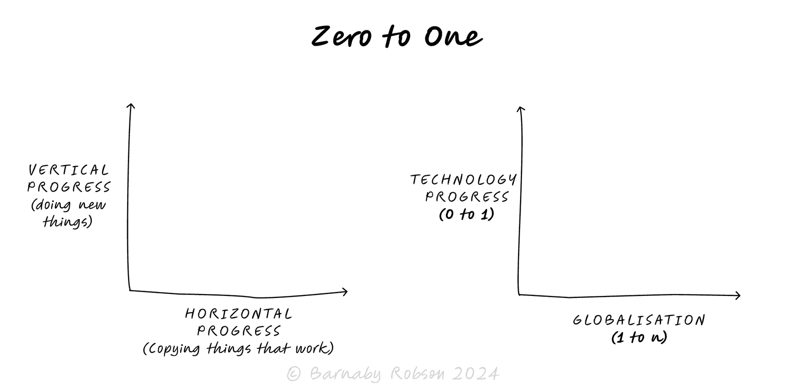
Aim for vertical progress—create something truly new (0 → 1), not just more of the same (1 → n). Win by building a monopoly on a focused niche and compounding from there.