Law of Diminishing Returns
Each extra unit adds less benefit beyond a point; invest until marginal benefit ≈ marginal cost.
Author
Classical microeconomics (Turgot, Menger, Marshall)
Model type
Each extra unit adds less benefit beyond a point; invest until marginal benefit ≈ marginal cost.
Classical microeconomics (Turgot, Menger, Marshall)
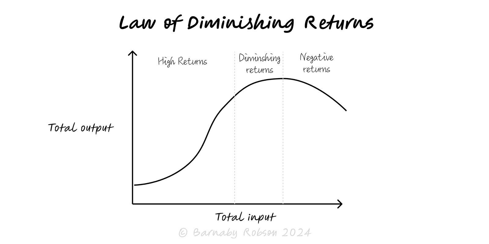
The law of diminishing returns says that holding other factors fixed, adding more of one input eventually produces smaller marginal output. Early on you may see increasing returns (set-up effects, learning), but the response curve turns concave as congestion, interference and limits bite. Related but separate: diminishing marginal utility in consumption (each extra unit feels less valuable than the last).
Fixed + variable inputs – with one factor fixed (e.g., capacity), the marginal product of the variable factor falls after a threshold.
Marginal vs average – the marginal line turns down before the average; when marginal < average, the average starts to fall.
Sources of decline – congestion (too many people/machines), scarce complements (tooling, attention), coordination overhead, fatigue.
S-curve dynamics – early acceleration → middle diminishing returns → late saturation.
Utility analogue – in demand/UX, extra features or messages add less incremental value and can even harm.
Marketing spend – extra budget buys smaller incremental conversions after prime audiences are reached.
Staffing & queues – more agents cut wait times at first; later additions barely move the needle.
Performance tuning – more compute/threads help until I/O, locks or latency dominate.
Product scope – feature additions bring less adoption; risk of bloat and complexity.
Hours worked – overtime boosts output initially, then errors and rework rise.
Pricing & promos – deeper discounts pull fewer extra buyers and erode margin.
Define driver and outcome – e.g., ad £ vs incremental conversions; headcount vs lead time.
Measure in increments – test stepped increases; compute marginal gain per last unit (Δoutput/Δinput).
Fit a simple response curve – concave or S-curve; visualise marginal and average lines.
Choose the operating point – increase input until MB = MC (or until your target service level/ROI threshold).
Stage spend/capacity – add in tranches with review gates; stop when marginal ROI falls below the hurdle.
Reset the curve by lifting constraints – fix bottlenecks (tooling, training, architecture); a new, higher-ceiling curve may emerge.
Re-estimate periodically – mix, seasonality and competition shift the response.
Optimising on averages – decisions must use marginal gains, not average ROI.
Assuming concavity everywhere – some domains have increasing returns (network effects, learning curves) before diminishing sets in.
Attribution errors – noisy measurement overstates or hides diminishing returns; use hold-outs and proper baselines.
Hidden complements – starving a complementary input (QA, onboarding) creates faux diminishing returns.
End-of-curve thrash – piling on inputs at saturation wastes cash and creates complexity.
Static mindset – the point of diminishing returns moves as constraints change.
Click below to learn other mental models

Before building, map the space: the key forks, dead ends and dependencies—so you can choose a promising path and run smarter tests.

When a rising power threatens to displace a ruling power, fear and miscalculation can tip competition into conflict unless incentives and guardrails are redesigned.

Aim for vertical progress—create something truly new (0 → 1), not just more of the same (1 → n). Win by building a monopoly on a focused niche and compounding from there.